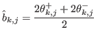
next up previous contents
Next: Special nasty cases Up: How are different positions Previous: Observables   Contents


Basic binning

1.
We have several patterns, say $ P$ . Each $ k$ -th pattern, for $ k=1,\ldots,P$ , is constituted by $ N_k$ angular intervals in the diffraction angle $ 2\theta\equiv{\ensuremath{{2\theta}}}$ :

$\displaystyle b_{k,j}={\ensuremath{\left[{{\ensuremath{{2\theta}}}_{k,j}^{-},{\ensuremath{{2\theta}}}_{k,j}^{+}}\right]}},\qquad j=1,\ldots,N_k
$

of center

$\displaystyle \hat{b}_{k,j}={\ensuremath{\displaystyle{\frac{{\ensuremath{\disp...
...{+}+{\ensuremath{{2\theta}}}_{k,j}^{-}}}}}{{\ensuremath{\displaystyle{2}}}}}}}
$

and width

$\displaystyle {\ensuremath{\left\vert{b_{k,j}}\right\vert}}={\ensuremath{{2\theta}}}_{k,j}^{+}-{\ensuremath{{2\theta}}}_{k,j}^{-}
$

To each interval is associated a counting $ C_{k,j}$ , an efficiency correction factor $ e_{k,j}$ , a monitor $ m_{k,j}$ (ionization chamber times acquisition time). All 'bad' intervals have been already flagged down and discarded. Efficiency corrections and monitors are supposed to be normalized to a suitable value. Note that intervals $ b_{k,j}$ might have multiple overlaps and might not cover an compact angular range.
2.
Following Mighell's statistics[6] and normal scaling procedures, we first transform those numbers into associated intensities, intensity rates and relevant s.d.:

$\displaystyle I_{k,j}={\ensuremath{\displaystyle{\frac{{\ensuremath{\displaysty...
...nsuremath{\left({C_{k,j}+\min{\ensuremath{\left({1,C_{k,j}}\right)}}}\right)}}
$

$\displaystyle \sigma_{I_{k,j}}={\ensuremath{\displaystyle{\frac{{\ensuremath{\d...
...ath{\displaystyle{m_{k,j}}}}}}}}\sqrt{{\ensuremath{\left({C_{k,j}+1}\right)}}}
$

$\displaystyle r_{k,j}={\ensuremath{\displaystyle{\frac{{\ensuremath{\displaysty...
...nsuremath{\left({C_{k,j}+\min{\ensuremath{\left({1,C_{k,j}}\right)}}}\right)}}
$

$\displaystyle \sigma_{r_{k,j}}={\ensuremath{\displaystyle{\frac{{\ensuremath{\d...
...k,j}}\right\vert}}m_{k,j}}}}}}}}\sqrt{{\ensuremath{\left({C_{k,j}+1}\right)}}}
$

3.
We set up the final binned grid, composed of $ M$ binning intervals

$\displaystyle B_\ell=[{\ensuremath{{2\theta}}}_0+(\ell-1)B, {\ensuremath{{2\theta}}}_0+\ell B],\qquad \ell=1,\ldots,M
$

all contiguous and each having the same width

$\displaystyle {\ensuremath{\left\vert{B_\ell}\right\vert}}=B$

and each centered in

$\displaystyle \hat{B}_\ell={\ensuremath{{2\theta}}}_0+(\ell-1/2)B,$

covering completely the angular range between $ {\ensuremath{{2\theta}}}_0$ and $ {\ensuremath{{2\theta}}}_{max}={\ensuremath{{2\theta}}}_0+MB$ .
4.
For bin $ \ell$ , we consider only and all the experimental intervals

$\displaystyle b_{k,j}$   such that$\displaystyle \qquad {\ensuremath{\left\vert{ b_{k,j}\cap B_\ell }\right\vert}} > 0.
$

More restrictively, one may require to consider only and all the experimental intervals

$\displaystyle b_{k,j}$   such that$\displaystyle \qquad \hat{b}_{k,j}\in B_\ell .
$

5.
In order to estimate the rate in each $ \ell$ -th bin, we use all above selected rate estimates concerning bin $ B_\ell$ and we get a better one with the weighted average method.
In the weighted average method, we suppose to have a number $ N_E$ of estimates $ O_n$ of the same observable $ O$ , each one with a known s.d. $ \sigma_{O_n}$ and each (optionally) repeated with a frequency $ \nu_n$ . Then

$\displaystyle \langle O\rangle ={\ensuremath{\displaystyle{\frac{{\ensuremath{\...
...remath{\displaystyle{
\mathop{\sum}_{n=1}^{N_E}\nu_n
\sigma_{O_n}^{-2}
}}}}}}}
$

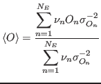
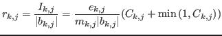
Clearly the place of the frequencies in our case can be taken by coefficients

$\displaystyle {\ensuremath{\displaystyle{\frac{{\ensuremath{\displaystyle{{\ens...
...ert{ b_{k,j}\cap B_\ell }\right\vert}}}}}}{{\ensuremath{\displaystyle{B}}}}}}}
$

that weigh the $ k,j$ -th estimate by its relative extension within bin $ B_\ell$ .
6.
Now we can simply accumulate registers

$\displaystyle X_\ell=\mathop{\sum_{k,j}}_{ {\ensuremath{\left\vert{ b_{k,j}\cap...
...aystyle{B}}}}}}}\ r_{k,j}\ {\ensuremath{\left({\sigma_{r_{k,j}}}\right)}}^{-2}
$

and

$\displaystyle Y_\ell=\mathop{\sum_{k,j}}_{ {\ensuremath{\left\vert{ b_{k,j}\cap...
...th{\displaystyle{B}}}}}}}\ {\ensuremath{\left({\sigma_{r_{k,j}}}\right)}}^{-2}
$

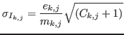
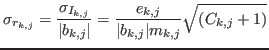
so that we can extract an intensity rate estimate (counts per unit diffraction angle and per unit time at constant incident intensity) as

$\displaystyle R_\ell={\ensuremath{\displaystyle{\frac{{\ensuremath{\displaystyle{X_\ell}}}}{{\ensuremath{\displaystyle{Y_\ell}}}}}}};
$

$\displaystyle \sigma_{R_\ell}={\ensuremath{\displaystyle{\frac{{\ensuremath{\displaystyle{1}}}}{{\ensuremath{\displaystyle{\sqrt{Y_\ell}}}}}}}}.
$

Now optionally we can transforms rates in intensities (multiplying both $ R_\ell$ and $ \sigma_{R_\ell}$ by $ B$ ). We can use any other scaling factor $ K$ as we wish instead of $ B$ . The best cosmetic scaling is the one where

$\displaystyle \mathop{\sum}_{\ell=1}^M{\ensuremath{\displaystyle{\frac{{\ensure...
...\displaystyle{R_\ell}}}}{{\ensuremath{\displaystyle{\sigma_{R_\ell}^2}}}}}}}=M
$

as if the intensities were simply counts. Therefore $ K$ is given by

$\displaystyle K={\ensuremath{\displaystyle{\frac{{\ensuremath{\displaystyle{
1
...
...h{\displaystyle{R_\ell}}}}{{\ensuremath{\displaystyle{\sigma_{R_\ell}^2}}}}}}}
$

In output then we give 3-column files with columns

$\displaystyle \hat{B}_\ell, \quad KR_\ell, \quad K\sigma_{R_\ell}
$


Subsections
next up previous contents
Next: Special nasty cases Up: How are different positions Previous: Observables   Contents
Thattil Dhanya 2019-04-08