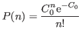
If we have a count value ![]() that follows a Poisson distribution,
we can assume immediately that the average is
that follows a Poisson distribution,
we can assume immediately that the average is ![]() and the s.d. is
and the s.d. is
![]() .
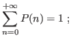
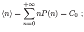
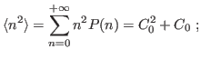
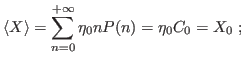
I.e., repeated experiments would give values
.
I.e., repeated experiments would give values ![]() distributed according to the normalized distribution
distributed according to the normalized distribution
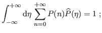
This obeys
Suppose now that our observable is
where
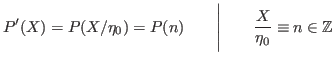
and now,
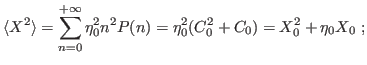
Now it is no more valid that
that is the characteristic relationship for a normal-variate distribution.
Moreover, assume now that the scaling factor is not exctly known
but instead it is a normal-variate itself with average ![]() , s.d.
, s.d.
![]() , and distribution
, and distribution
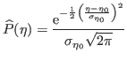
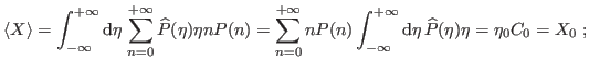
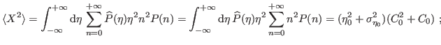
Then,

where in the last we discard, as usual, the 4th order in the relative errors. Both the exact and approximated forms are exactly the same as if both distributions were to be normal.