First we give an analytical comparison between simple average and Mighell-Poisson weighted average
for
![]() .
If the two events are
.
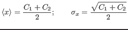
If the two events are ![]() and
and ![]() , then
, then
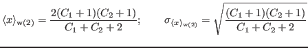
For the M-P weighted average,
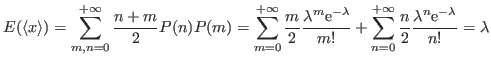
Now, supposing that the common 'true' value of ![]() is
is ![]() ,
we use the Poisson distribution to compare the expectation values of the two results. The expectation value of the simple average is
,
we use the Poisson distribution to compare the expectation values of the two results. The expectation value of the simple average is
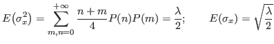
As expected, the simple average gives the true value. For its variance,
In order to evaluate the difference with the M-P weighted average, we rewrite the latter as
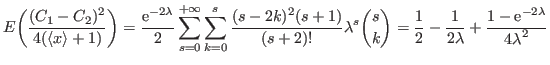
and calculate the expectation value of the last term:
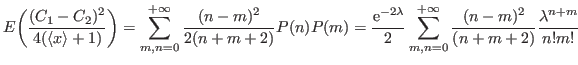
Rearranging the sums with
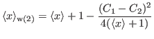
So, the relative difference between averages is
The relative error on
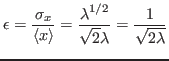
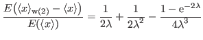
therefore
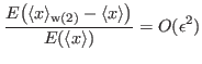
Therefore, the expectation value of the error (relative) involved in taking the M-P weighted average instead of the simple average is negligible.